Open source

EvoAgent-NO: Agents that evolve what a physics computer learns

An open-source engine that pretrains neural operators with zero data: a program poses physics problems, an exact solver answers them, and LLM agents rewrite the program when the operator stops learning.

2026-09-27 · 8 min · Chips & Superintelligence Labs

A neural operator is a physics computer. Give it a field and it returns the next one, or the solution, in a single forward pass instead of a solver run. How do you pretrain one when you have no data?

The usual answer is to run a solver in advance over a fixed family of PDEs, parameters and initial conditions, and train on whatever comes out. Someone has to choose those problems before training starts. They pick coefficient ranges, amplitudes, boundary conditions, and the operator never gets a say in what it learns next. If the choice is off, the compute goes to problems that are too easy, too hard, or beside the point, and nobody finds out until the model is tested.

EvoAgent-NO is our attempt at letting the system make that choice. It is open source, Apache-2.0, and on GitHub.

The idea

A small Python program poses physics problems. An exact solver answers them on the GPU. A neural operator, which we call the student, trains on the answers. When the student stops improving, LLM agents rewrite the program that poses the problems, and a rewrite is kept only if a short trial shows the student learns more from it.

You write the first version of the program. It does not need to be good. Nothing is downloaded.

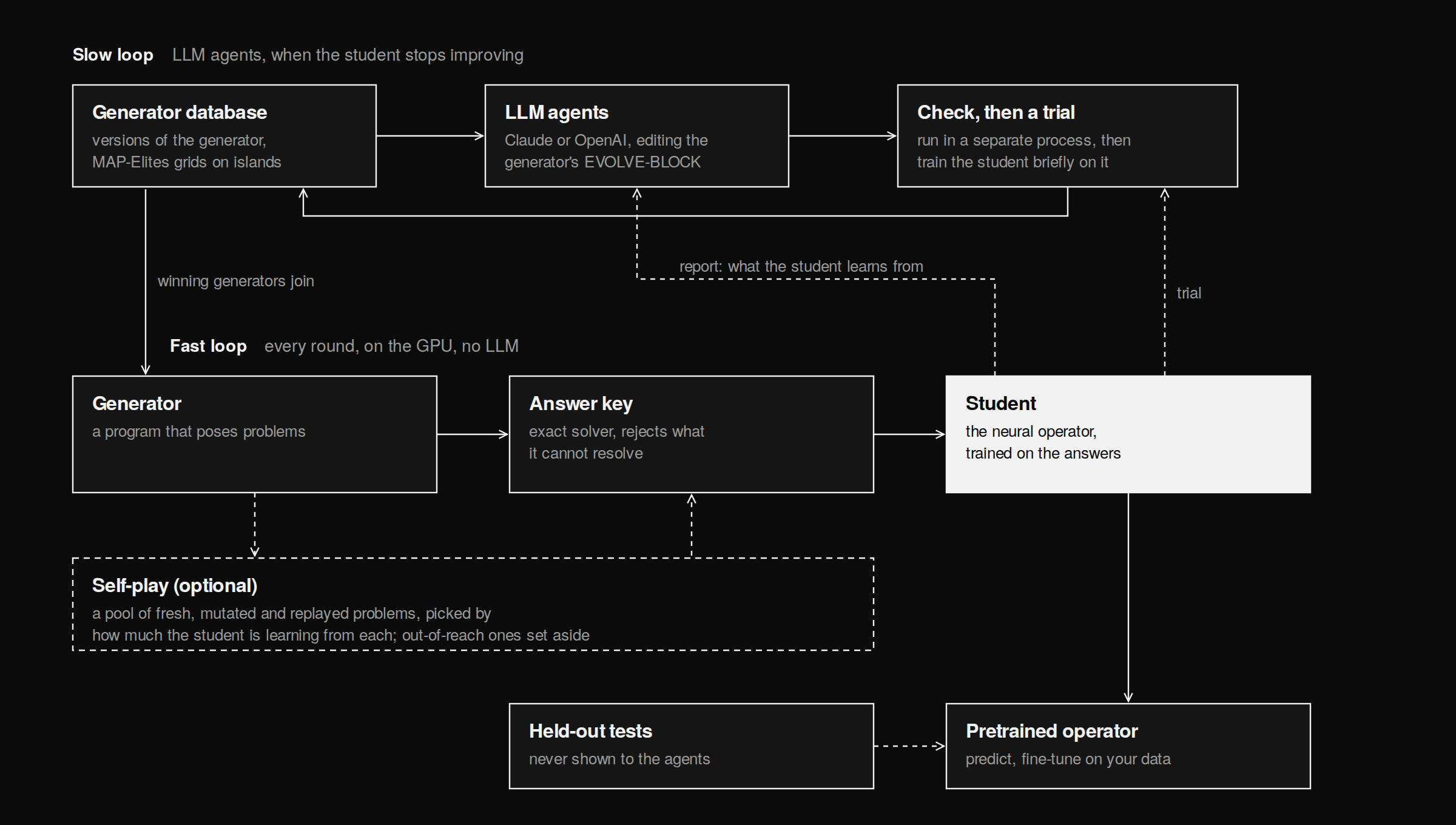
The two loops of EvoAgent-NO. The fast loop runs every round on the GPU: the generator poses problems, the answer key solves them, the student trains. The slow loop runs when the student stops improving: LLM agents edit the generator, each edit is checked and then tried on the student, and winning generators join the fast loop. Self-play inside the fast loop is optional.

There are two loops, running at very different speeds.

The fast loop

Every round, on the GPU, with no LLM involved:

The generator is a Python program with two functions, generate_problems(rng, n) and mutate_problem(problem, rng). It decides which equations, coefficients and initial conditions exist.
The answer key is an exact solver. It solves every problem twice, at two resolutions, and drops anything it cannot answer reliably: blow-ups, and problems where the two solutions disagree. The student is never graded against a wrong answer.
The student is a Fourier neural operator in 1D, 2D or 3D. It sees input fields and predicts the output field without being told which equation produced them. It is the only part that trains, and it is what you keep at the end.

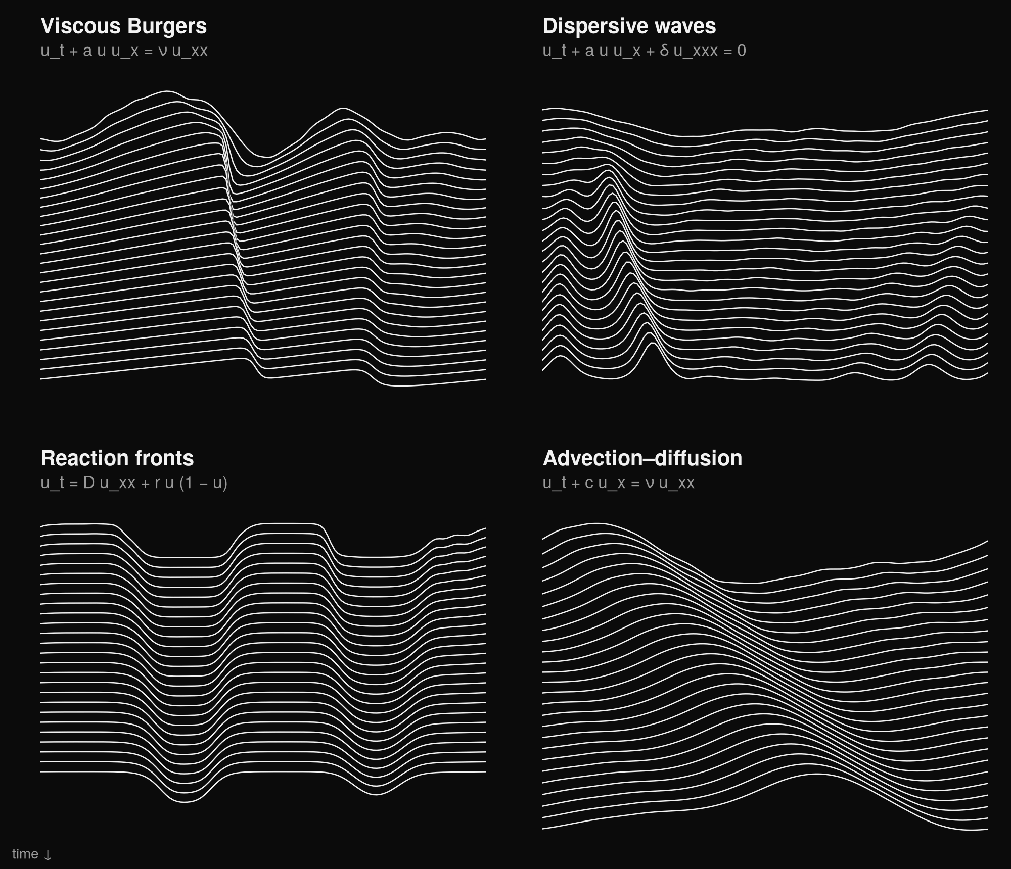
Four problems posed by the 1D template and solved by its answer key: viscous Burgers steepening into a shock, a dispersive wave train, reaction fronts, and a field carried and spread by advection–diffusion. Each line is one frame; time runs down.

Four problems the 1D template can pose, as its answer key solved them. Each line is one frame and time runs down. The student sees four frames and predicts the next, without being told which equation it is looking at.

The slow loop

When the student's training loss stops improving, the slow loop wakes up:

A database of generators. Every version the agents have written, kept in MAP-Elites grids on a few islands, so different kinds of generator survive side by side.
LLM agents. Claude or an OpenAI model gets the physics description, a parent generator, a few others for ideas, and a report of what the student has been learning from. It replies with SEARCH/REPLACE edits to the part of the generator marked as evolvable. It never sees the held-out tests.
Check, then a trial. Each edit runs in a separate process with a time limit and has to produce well-formed problems. Then the student trains on half of the new generator's problems for one round, and the score is how much error that removed on the other half. The student is put back exactly as it was.
What the student trains on. Your generator, always, plus every rewrite that beat it in the latest trial, in equal shares.

What an agent's edit looks like

Here is a real one. We started a run from a generator that only knew the heat equation:

def generate_problems(rng, n):
    """n heat-equation problems with random diffusivity and random initial fields."""
    return [Problem(coef=_heat(math.exp(rng.uniform(math.log(1e-3), math.log(0.3)))), ...)
            for _ in range(n)]

At its first evolution step, Claude Sonnet 5 read the physics description and the training report, and replied with this summary and a SEARCH/REPLACE edit:

Replaced the pure-diffusion generator with one that samples across all PDE term families, each parameterized near but inside the stability limits.

Part of what it wrote:

_FAMILIES = (
    "diffusion", "advection", "dispersion", "hyperdiff",
    "burgers", "reaction", "burgers_reaction", "forced",
)
_FAMILY_WEIGHTS = np.array([0.10, 0.15, 0.15, 0.10, 0.15, 0.15, 0.10, 0.10])

def _sample_family(name, rng):
    ...
    elif name == "burgers":
        nu = _log_uniform(rng, 1e-2, 0.3)
        a = rng.uniform(-5.0, 5.0)
        coef = _coef(diffusion=nu, burgers=a)
        amp = _log_uniform(rng, 0.3, 2.5)

The edit ran in a separate process, produced well-formed problems and won its trial. Nobody told the agent which physics to add: it had the equation the answer key can solve and the report of what the student was learning from.

The idea of LLMs evolving programs against an automatic evaluator comes from AlphaEvolve. The difference here is what the programs are for and who evaluates them. The programs pose questions rather than answer them, and the evaluator is a student that keeps learning.

Three design decisions

Measure a new generator; do not extrapolate. The self-play paper that inspired this project, Cowsik et al., Self-Play Pretraining with Zero Data (arXiv 2609.30063), ranks problems by learning progress: how well a problem's gradient lines up with the direction the student has been moving. That works well inside a round. It cannot see physics the student has never trained on, which is exactly what a new generator is for. So a candidate generator gets a short training trial instead, and its score is error that actually went away.

Add, do not replace. Without data there is no direct measure of the thing we want, a student that generalizes to physics it has not seen. The trial is a stand-in, and stand-ins can mislead: a generator whose problems are narrow and easy can win a trial and still be a poor curriculum. So a winning rewrite joins your generator instead of replacing it. The student keeps training on what you wrote, and a misleading trial can cost at most its share.

The evaluator moves. A generator's score is measured on the current student, and the student keeps learning, so scores go stale. They fade every step, and your generator and the strongest rewrites are measured again before the agents see them.

Self-play, if you want it

With --selfplay, a pool also picks the problems within each round, as in the paper: fresh ones from the generator, mutations of the problems the student is learning from fastest, and replays with new random fields. Learning progress is computed for the whole batch in one forward-mode pass. Problems far harder than the generator's typical one are set aside as out of reach, so a handful of extreme problems cannot dominate the gradient. It is off by default.

What you can use it for

EvoAgent-NO is for the situation where you can simulate something but do not have, or cannot afford, a large dataset of simulations to train a neural operator on. Some examples:

A fast surrogate before you have data. You will run the same kind of simulation thousands of times, for design sweeps, inverse problems, uncertainty studies or control, and want a neural operator that answers in milliseconds. Pretrain it here on problems your solver generates, then finetune it on the handful of real or high-fidelity runs you do have.
You know the equation, not the distribution. You can write the PDE and a solver, but not which coefficients, amplitudes and initial conditions matter. Write a rough generator that draws from wide ranges and let the agents shape it. The broad-guess example starts this way.
From one case to a family. Your solver is set up for one regime, one material or one kind of term. The agents can extend the generator to the rest of what the solver supports. The heat-only example starts from pure diffusion.

Closer to what we work on at the lab:

Use case	Physics	Start from
Steady thermal map of a die: power map in, temperature out	−∇·(k∇T) = q, conductivity by material	the `elliptic2d` template; your own backend in 3D
Transient heating through a package	the 3D heat equation	the `heat3d` example
Potential in layered dielectrics, IR drop across a power grid	−∇·(σ∇φ) = f with a two-phase σ	the `elliptic2d` template
Dopant diffusion during anneal, moving fronts in process models	diffusion–reaction	the `pde1d` template, or your own backend
Mask to aerial image in computational lithography	an imaging model	your own physics backend

And beyond chips: flow through porous media and groundwater (Darcy's law is the elliptic2d equation, with permeability for a), heat transfer in composites, reaction–diffusion in chemistry and biology, and wave and transport problems with a backend of your own. For research on curricula themselves, every run keeps each generator the agents wrote, its trial score and the report the agents saw.

Using it

pip install git+https://github.com/chipsuperintelligence/EvoAgent-NO
evoagent-no new pde1d tasks/my-pde          # a task folder from a template
evoagent-no check tasks/my-pde              # wired up? seconds
evoagent-no run tasks/my-pde                # agents evolve the generator as the student trains
evoagent-no run tasks/my-pde --no-agents    # the baseline: your generator as written
evoagent-no finetune runs/my-pde/agents-s0 --data mine.npz

Or from Python:

import evoagent_no as evo

evo.run("tasks/my-pde", "runs/my-pde/agents-s0")
student = evo.load_student("runs/my-pde/agents-s0")
prediction = student.predict(inputs)
student.finetune(my_inputs, my_targets, steps=500)

Two templates ship with it: pde1d, time stepping on 1D PDEs built from nine terms (advection, diffusion, dispersion, Burgers, reaction and more), and elliptic2d, steady diffusion −∇·(a∇u) = f in 2D, an operator from coefficients and sources to solutions. Two more examples, transport in 1D and heat in 3D, bring their own physics, and two more start the built-in 1D physics from a different generator.

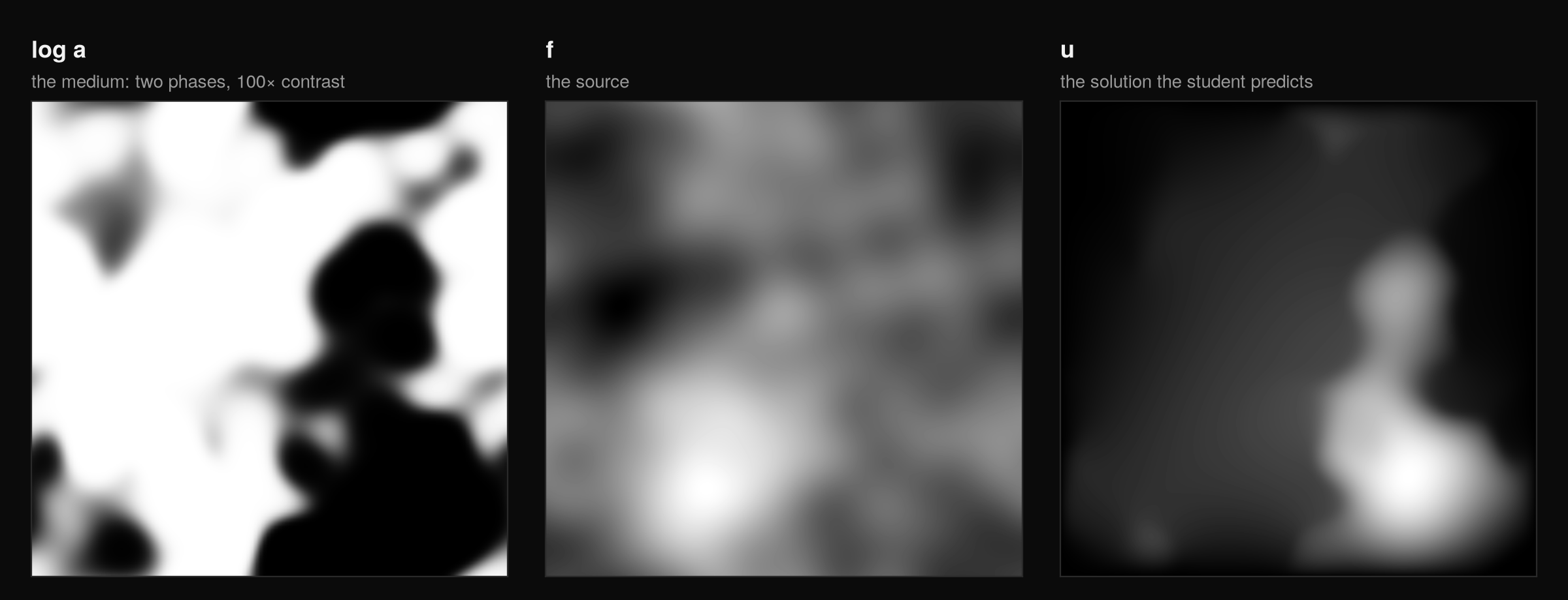
One problem from the 2D template: the log-coefficient of a two-phase medium with a hundredfold contrast, a varying source, and the solution u that the student learns to predict from the other two.

One problem from the 2D template. The student sees the medium and the source and predicts the solution; the answer key solved it at two resolutions and the two agreed.

Your own physics

Everything about a problem domain lives in one folder: task.yaml for the settings, generator.py for the first version of the question-maker, context.md for what the agents are told about the physics, and optionally your own physics.py and heldout.py.

A physics backend is a module with five things: a Problem dataclass, an IO description of what a sample looks like, check to reject malformed problems, describe to say what kind of problem it is, and solve, which turns a batch of problems into input and output fields on a regular grid. The student is built from IO, so a new backend needs no model code. IO can also state the equation's symmetries: for steady diffusion, doubling f doubles u, and scaling a scales u inversely, and the student is built so its answer scales the same way.

The LLM, and what it costs

The LLM only works in the slow loop, and only on code. It does not solve physics, train the student, score its own edits or run anything. EvoAgent-NO applies its edits, runs them in a separate process and measures them on the student.

By default the agents run Claude Sonnet 5 at medium reasoning effort through the Claude Code CLI, on your own login: a single, tool-free completion per call, with nothing to approve. The model, the effort level and a per-call budget are settings, and a list mixes models by weight. With the defaults, a 200-round run makes at most 18 calls, and fewer when the student is still improving, because the agents are only called once it has stopped.